What you need
Use an offline joint-angle plot with chosen start angle, end angle and duration. Avoid sending sampled positions directly to hardware.
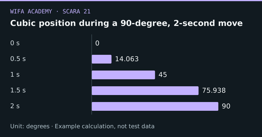
Read the diagram as a data table
| Condition or component | degrees |
|---|---|
| 0 s | 0 |
| 0.5 s | 14.063 |
| 1 s | 45 |
| 1.5 s | 75.938 |
| 2 s | 90 |
The calculation
s(u) = 3u² − 2u³; u=t/T
q(t) = q₀ + (q_f − q₀) × s(u)
T is total duration and 0≤u≤1. The joint displacement and q use a consistent angle or distance unit.
Worked example
A 90° move over 2 s reaches 14.0625° at 0.5 s, 45° at 1 s and 75.9375° at 1.5 s. Peak speed is 1.5×90/2 = 67.5°/s, so duration must respect the axis speed limit.
Try it step by step
- Choose endpoint conditions and calculate the required peak velocity and acceleration before selecting duration.
- Sample the function offline and plot position, velocity and acceleration for inspection.
- Synchronize multiple joints using a common duration chosen for the most restrictive axis.
- Use a trajectory interface that enforces machine limits and validate the resulting motion in simulation before physical commissioning.
How to check the result
The first and last position must match the requested endpoints, and the derived velocity must be zero at both ends.
Common mistake to avoid
Zero endpoint velocity does not mean zero endpoint acceleration. A quintic time law is needed when both must vanish in this polynomial family.
Reference reading
Primary references for the underlying models, APIs or application context. The worked numbers and plots above are educational calculations, not results reported by these sources.