What you need
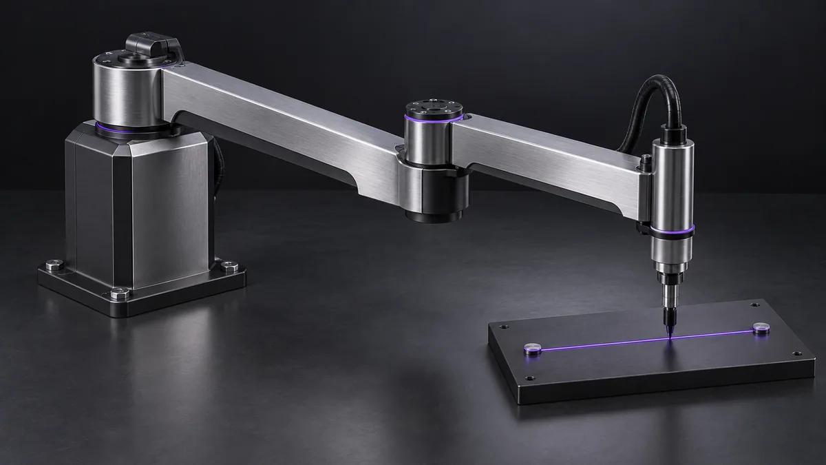
Use a two-link simulator, a chosen start and end point and a consistent inverse-kinematics branch.
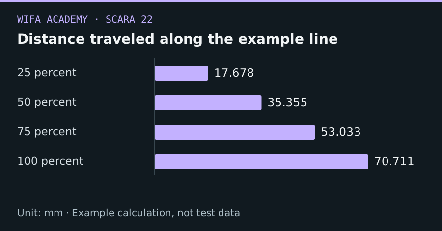
Read the diagram as a data table
| Condition or component | mm |
|---|---|
| 25 percent | 17.678 |
| 50 percent | 35.355 |
| 75 percent | 53.033 |
| 100 percent | 70.711 |
The calculation
p(s) = (1 − s)p_start + s p_end, 0≤s≤1
p is an x-y position vector. A separate time law s(t) sets the speed; geometric interpolation alone does not define motion timing.
Worked example
From (100,100) to (150,50) mm, the midpoint is (125,75) mm and path length is √(50²+50²)=70.71 mm. Check every sampled point for reachability and joint-speed amplification, not only the two endpoints.
Try it step by step
- Sample the Cartesian segment and reject unreachable or colliding points with the full tool geometry included.
- Solve a continuous inverse-kinematics branch and inspect joint-angle plots for jumps.
- Apply a time law, calculate joint rates and accelerations, and increase duration or replan if any axis exceeds limits.
- Compare the simulated executed path with the intended line and document interpolation tolerances.
How to check the result
Measure maximum perpendicular deviation from the requested line across the complete path.
Common mistake to avoid
A collision-free line for the tool tip may still sweep an elbow through an obstacle. Endpoint-only checks miss this problem.
Reference reading
Primary references for the underlying models, APIs or application context. The worked numbers and plots above are educational calculations, not results reported by these sources.