What you need
Use an offline motion plot with known distance, maximum speed and acceleration. Keep all units consistent.
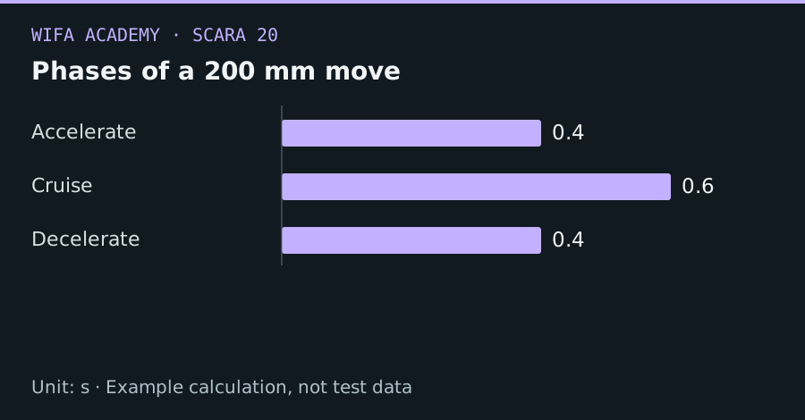
Read the diagram as a data table
| Condition or component | s |
|---|---|
| Accelerate | 0.4 |
| Cruise | 0.6 |
| Decelerate | 0.4 |
The calculation
t_acc = v_max / a
d_acc_total = v_max² / a
t_total = 2t_acc + (d − d_acc_total)/v_max
The expression applies when d≥d_acc_total with zero initial and final speeds and symmetric acceleration.
Worked example
For d=0.2 m, v_max=0.2 m/s and a=0.5 m/s², acceleration lasts 0.4 s on each side. Acceleration and braking cover 0.08 m; the remaining 0.12 m cruises for 0.6 s. Total time is 1.4 s.
Try it step by step
- Check whether the distance supports a cruise segment; otherwise switch to the triangular case.
- Generate position, velocity and acceleration samples and verify continuity of position and velocity at phase boundaries.
- Compare peak demands with the axis and transmission limits, including load-dependent torque.
- Use the controller’s supported motion profile and compare its actual timing with this idealized baseline.
How to check the result
Integrating the velocity profile should reproduce the requested distance and end at zero speed.
Common mistake to avoid
Acceleration changes instantaneously in this ideal model. Flexible mechanisms may need a jerk-limited profile to reduce vibration.
Reference reading
Primary references for the underlying models, APIs or application context. The worked numbers and plots above are educational calculations, not results reported by these sources.