What you need
Use a known pose, a planar force vector and the validated Jacobian. Start with an offline calculation.
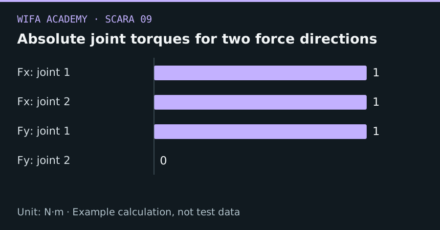
Read the diagram as a data table
| Condition or component | N·m |
|---|---|
| Fx: joint 1 | 1 |
| Fx: joint 2 | 1 |
| Fy: joint 1 | 1 |
| Fy: joint 2 | 0 |
The calculation
τ = Jᵀ × F
F is a planar force vector in N and τ is joint torque in N·m when J uses meters.
Worked example
At J=[[-0.1,-0.1],[0.1,0]], a force (10,0) N gives torques (-1,-1) N·m. A force (0,10) N gives (1,0) N·m. Equal force magnitudes load the joints differently depending on direction.
Try it step by step
- Define whether F is the force applied by the tool or to the tool and keep that sign convention consistent.
- Calculate torques at several path poses, especially those with large lever arms.
- Add the separate dynamic, friction and vertical-axis contributions required by the full mechanism model.
- Compare continuous and peak torque demands with motor, transmission and thermal limits, then validate the design safely.
How to check the result
Check the static result using a simple moment-arm calculation at a pose where the geometry is obvious.
Common mistake to avoid
SCARA horizontal-axis gravity loading differs from a vertical-plane arm, but bearings and structure still carry weight. This planar equation does not model those loads.
Reference reading
Primary references for the underlying models, APIs or application context. The worked numbers and plots above are educational calculations, not results reported by these sources.