What you need
Use a validated Jacobian in an offline numerical script. Avoid matrix inversion close to a singularity.
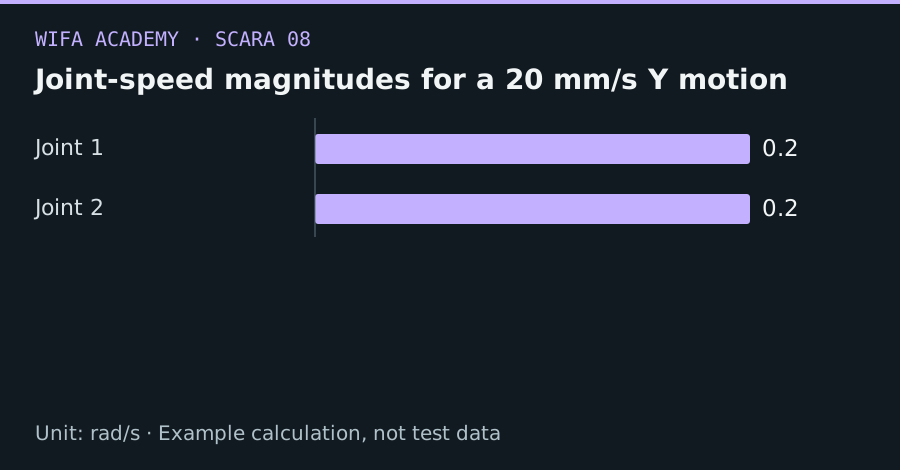
Read the diagram as a data table
| Condition or component | rad/s |
|---|---|
| Joint 1 | 0.2 |
| Joint 2 | 0.2 |
The calculation
q̇ = J⁻¹ × v
This direct inverse applies only to a nonsingular square Jacobian. Joint rates are rad/s when lengths and velocities use meters.
Worked example
At the right-angle pose with J=[[-0.1,-0.1],[0.1,0]], a desired velocity (0,0.02) m/s requires q̇₁=0.2 rad/s and q̇₂=-0.2 rad/s. Both joints move even though the target velocity is purely vertical in the drawing.
Try it step by step
- Evaluate the Jacobian at the current pose using the same conventions as the forward model.
- Solve the linear system and compare each requested joint rate with the configured machine limit.
- Scale the task velocity or replan where the solution exceeds limits, while preserving direction only when appropriate to the task.
- Check acceleration and continuity between samples; individually valid rates can still form an infeasible trajectory.
How to check the result
Multiplying the resulting rates by J should recover the requested velocity within numerical tolerance away from singularities.
Common mistake to avoid
Never use this local linear relation as a complete collision-aware motion planner. Large time steps invalidate the small-motion approximation.
Reference reading
Primary references for the underlying models, APIs or application context. The worked numbers and plots above are educational calculations, not results reported by these sources.