What you need
Use a calculator or a short offline script with angles in radians and lengths in meters.
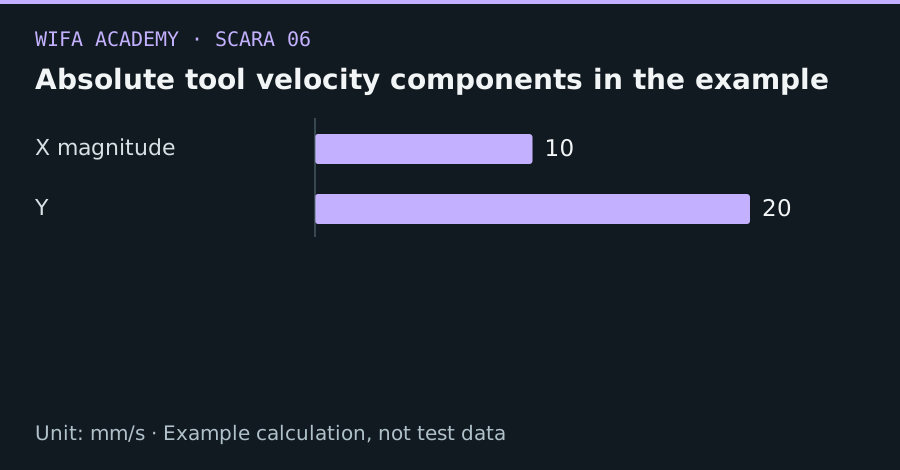
Read the diagram as a data table
| Condition or component | mm/s |
|---|---|
| X magnitude | 10 |
| Y | 20 |
The calculation
J = [[−L₁sinθ₁−L₂sin(θ₁+θ₂), −L₂sin(θ₁+θ₂)],
     [ L₁cosθ₁+L₂cos(θ₁+θ₂),  L₂cos(θ₁+θ₂)]]
v = J × q̇
J has units m/rad, q̇ is rad/s and v is m/s. The planar model excludes vertical and wrist axes.
Worked example
Illustrative numbers. Replace them with your measured inputs.
At L₁=L₂=0.1 m, θ₁=0 and θ₂=90°, J=[[-0.1,-0.1],[0.1,0]]. Joint speeds (0.2,-0.1) rad/s produce tool velocity (-0.01,0.02) m/s.
Try it step by step
- Differentiate each x-y position expression with respect to each joint angle and arrange columns by joint order.
- Evaluate the matrix at simple poses and compare predicted directions with the drawing.
- Perturb one joint by a tiny angle and compare forward-kinematics displacement divided by that angle with the corresponding Jacobian column.
- Use the validated matrix to inspect velocity amplification along the intended path.
How to check the result
Finite-difference and analytic Jacobians should converge as the perturbation shrinks, until floating-point effects dominate.
Common mistake to avoid
Using millimeters in one function and meters in another creates a factor-of-1,000 error in force or velocity calculations.
Reference reading
Primary references for the underlying models, APIs or application context. The worked numbers and plots above are educational calculations, not results reported by these sources.