What you need
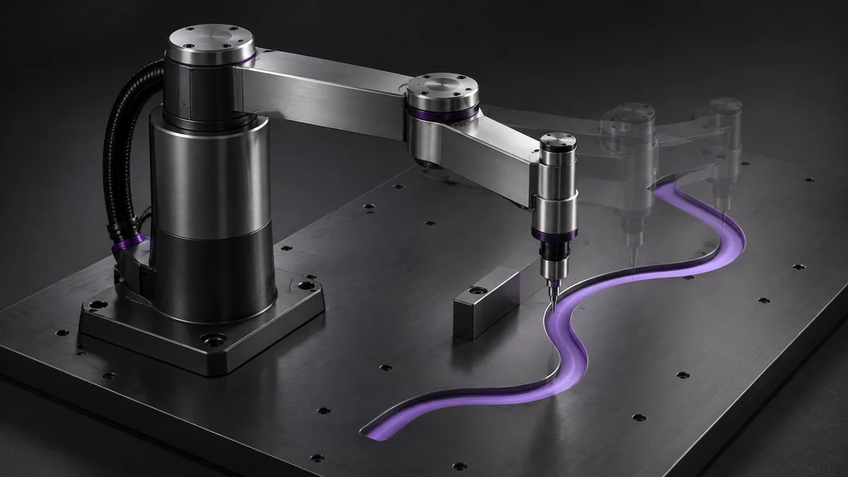
Use a sampled Cartesian path, both inverse-kinematics branches and explicit joint limits in a simulator.
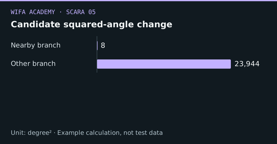
Read the diagram as a data table
| Condition or component | degree² |
|---|---|
| Nearby branch | 8 |
| Other branch | 23,944 |
The calculation
cost = Σ w_i × Δθ_i²
Δθ_i is the physically valid joint displacement from the previous state and w_i is a positive weighting. Handle angle wrapping according to actual travel limits.
Worked example
From previous angles (10°,70°), candidates (12°,68°) and (80°,-68°) have unweighted costs 8 and 23,944 degree². The first is locally smoother, but it still needs limit and collision checks.
Try it step by step
- Generate both inverse-kinematics candidates at each path point and reject invalid or colliding configurations first.
- Compute physically meaningful differences, respecting joints that cannot wrap continuously through 360°.
- Select the candidate with the smallest justified motion cost and retain it as the next reference.
- Inspect the whole path for singularities and branch dead ends; a greedy local choice may need a globally planned alternative.
How to check the result
Plot joint angle against path progress and inspect sudden jumps before adding any timing or drive commands.
Common mistake to avoid
The lowest cost is not necessarily collision-free or globally feasible. Never switch branches abruptly to escape a bad point while hardware is moving.
Reference reading
Primary references for the underlying models, APIs or application context. The worked numbers and plots above are educational calculations, not results reported by these sources.