What you need
Use shift records with planned production time, operating time, total count and good count. Define exclusions before recording data.
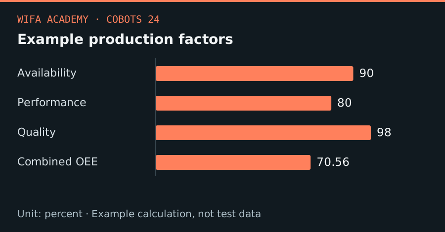
Read the diagram as a data table
| Condition or component | percent |
|---|---|
| Availability | 90 |
| Performance | 80 |
| Quality | 98 |
| Combined OEE | 70.56 |
The calculation
A = operating_time / planned_time
P = ideal_cycle × total_count / operating_time
Q = good_count / total_count
OEE = A × P × Q
A, P and Q are dimensionless fractions. Keep all time units consistent; the ideal cycle must be realistic and defined.
Worked example
For A = 0.90, P = 0.80 and Q = 0.98, the product is 0.7056, or 70.56%. Perfecting quality alone to 100% gives 72%, while raising performance to 90% with the original quality gives 79.38%.
Try it step by step
- Define planned time and a justified ideal cycle before the pilot; changing the denominator can make results look artificially better.
- Collect downtime reasons, total parts and accepted parts using a consistent shift boundary.
- Calculate the three factors separately and investigate the largest recoverable loss rather than optimizing the robot in isolation.
- Repeat after one controlled change and compare good output under similar product mix, staffing and replenishment conditions.
How to check the result
The underlying counts and times should reproduce the reported score. If performance exceeds 100%, review the ideal-cycle definition and time accounting.
Common mistake to avoid
OEE is a diagnostic measure, not a financial return or safety metric. Comparing unlike product mixes without context is misleading.
Reference reading
Primary references for the underlying models, APIs or application context. The worked numbers and plots above are educational calculations, not results reported by these sources.