What you need
Use a stopwatch, a task video, a spreadsheet and representative parts. Observe the manual process without changing its safeguards.
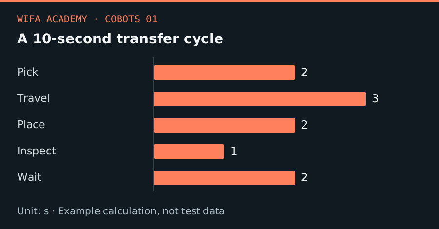
Read the diagram as a data table
| Condition or component | s |
|---|---|
| Pick | 2 |
| Travel | 3 |
| Place | 2 |
| Inspect | 1 |
| Wait | 2 |
The calculation
t_cycle = t_pick + t_move + t_place + t_check + t_wait
Q_ideal = 3600 / t_cycle
All times are seconds per part. Q_ideal is parts per hour before downtime, rejects and replenishment.
Worked example
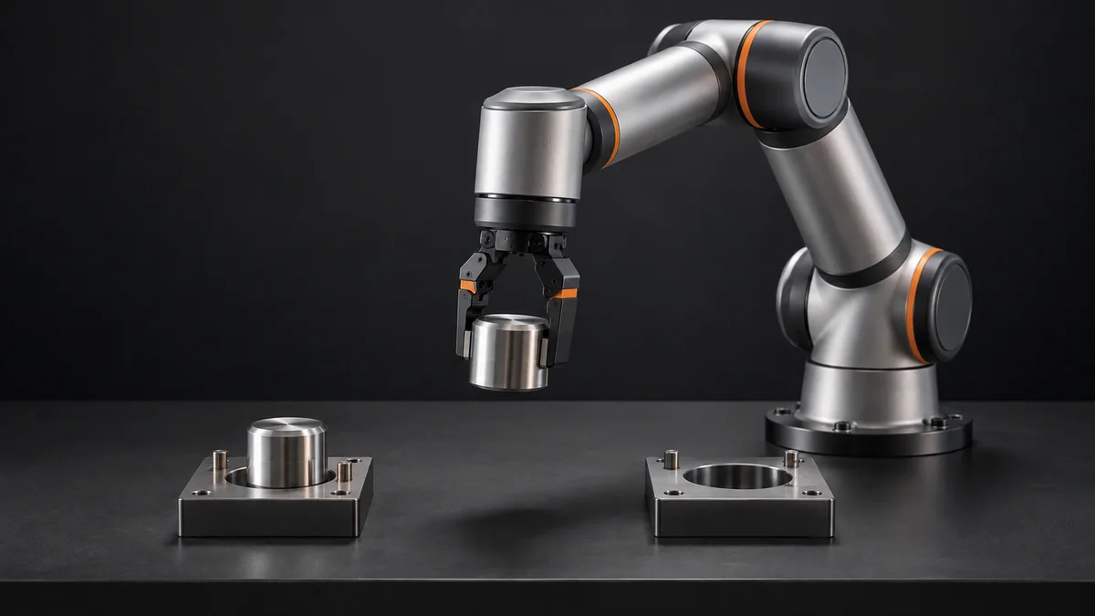
Suppose picking takes 2 s, travel 3 s, placement 2 s, inspection 1 s and waiting 2 s. The total is 10 s, giving 360 parts/h ideally. Removing one second of waiting gives 400 parts/h; doubling travel speed does not double output.
Try it step by step
- Record at least 20 consecutive cycles and mark where each step starts and ends; retain outliers instead of deleting them.
- Separate time that overlaps, such as camera processing during travel, from steps that must run sequentially.
- Create a conservative robot estimate using actual approach distances and gripper timing, not just an advertised cycle time.
- Draw replenishment and rejected-part handling into the sequence before deciding whether the task is a useful pilot.
How to check the result
Compare the model with a simulated sequence, then time a supervised pilot. Report median, slow cycles and good parts produced, not only the fastest cycle.
Common mistake to avoid
This sum assumes sequential steps. Summing overlapping durations exaggerates the cycle; ignoring operator replenishment understates it.
Reference reading
Primary references for the underlying models, APIs or application context. The worked numbers and plots above are educational calculations, not results reported by these sources.