What you need
Use repeated detections of a stationary reference and a validated mapping. Separate random variation from systematic calibration bias.
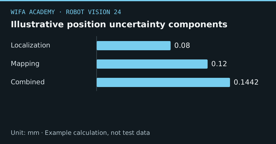
Read the diagram as a data table
| Condition or component | mm |
|---|---|
| Localization | 0.08 |
| Mapping | 0.12 |
| Combined | 0.1442 |
The calculation
σ_x ≈ |s| × σ_u
Σ_world ≈ J × Σ_pixel × Jᵀ
s is local mm/pixel, σ_u is pixel standard deviation and J is the local derivative of the coordinate mapping.
Worked example
At 0.1 mm/pixel, 0.8-pixel random localization scatter gives 0.08 mm standard uncertainty. If an independent mapping uncertainty is 0.12 mm, their root-sum-square is approximately 0.144 mm. A fixed bias must be treated separately.
Try it step by step
- Collect stationary detections without changing camera settings and estimate scatter in both image directions.
- Determine local mapping sensitivity at several workspace positions, not just the center.
- Combine compatible independent standard uncertainties and keep systematic offsets visible as separate terms.
- Validate the predicted uncertainty against held-out physical targets and reject regions that cannot meet the placement tolerance.
How to check the result
Report uncertainty assumptions, measurement conditions and observed bias alongside the estimated random spread.
Common mistake to avoid
Adding a calibration RMS in pixels directly to a robot error in millimeters is dimensionally wrong. Correlated uncertainties cannot be combined as independent terms.
Reference reading
Primary references for the underlying models, APIs or application context. The worked numbers and plots above are educational calculations, not results reported by these sources.