What you need
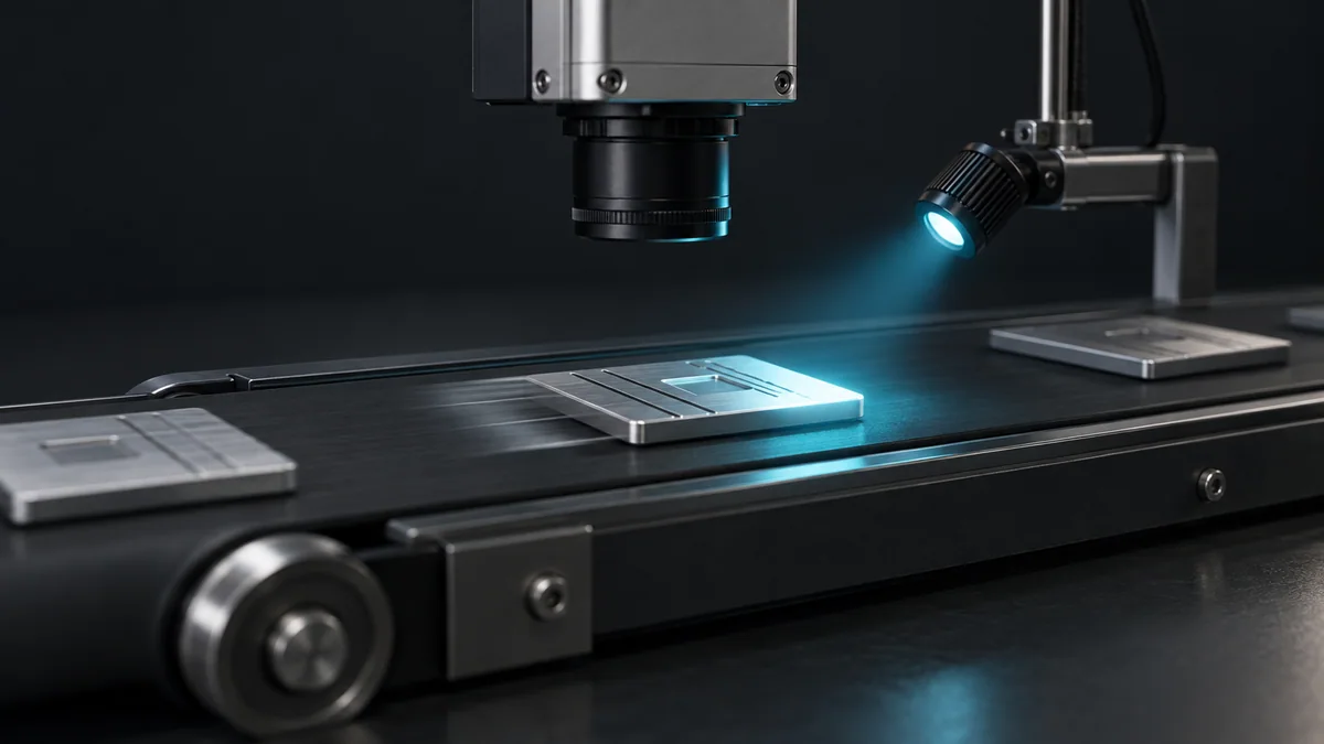
Use a moving calibration target, fixed camera, controlled light and timestamps. Begin with saved images rather than robot motion.
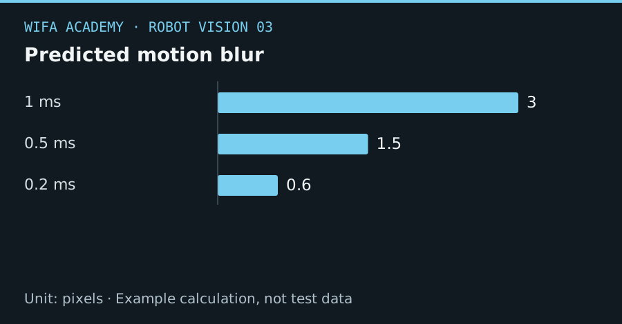
Read the diagram as a data table
| Condition or component | pixels |
|---|---|
| 1 ms | 3 |
| 0.5 ms | 1.5 |
| 0.2 ms | 0.6 |
The calculation
b_pixels = v × t_exp / s
v is object speed in mm/s, t_exp is exposure in s and s is mm/pixel at the object plane.
Worked example
At 300 mm/s and 0.1 mm/pixel, a 1 ms exposure gives 3 pixels of blur. A 0.2 ms exposure gives 0.6 pixels. To target at most one pixel in this simplified case, exposure must be no more than 0.333 ms.
Try it step by step
- Measure the fastest expected object speed and the pixel scale at the actual inspection plane.
- Calculate an exposure starting point and obtain adequate illumination without exceeding the camera or light’s operating limits.
- Compare captured edges at several exposures while keeping gain and image processing documented.
- Test detection and localization under the demanding motion condition, then record the complete exposure and trigger configuration.
How to check the result
Inspect real images for directional blur and measure localization spread. An apparent high frame rate does not prove a short exposure.
Common mistake to avoid
Rolling-shutter distortion is a different effect and may remain after reducing exposure. Extremely high gain can introduce noise that harms segmentation.
Reference reading
Primary references for the underlying models, APIs or application context. The worked numbers and plots above are educational calculations, not results reported by these sources.