What you need
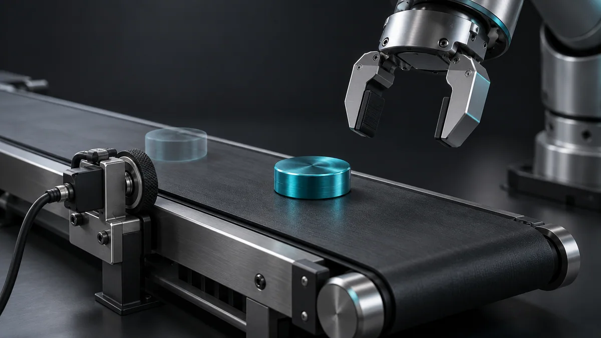
Use recorded detections, synchronized time data and a measured conveyor velocity or encoder signal. Simulate all target updates first.
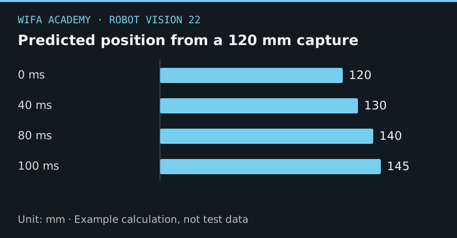
Read the diagram as a data table
| Condition or component | mm |
|---|---|
| 0 ms | 120 |
| 40 ms | 130 |
| 80 ms | 140 |
| 100 ms | 145 |
The calculation
x_now = x_capture + v × (t_now − t_capture)
x is conveyor-axis position in mm, v is signed mm/s and time is seconds. All positions must use the same frame.
Worked example
A part observed at 120 mm on a 250 mm/s belt is predicted at 140 mm after 80 ms. If actual latency is 100 ms but you assume 80 ms, the target is short by 5 mm.
Try it step by step
- Establish the conveyor axis direction in robot coordinates and verify the sign using a recorded forward movement.
- Associate each detection with exposure time rather than network receipt time, and synchronize clocks or use a documented common timing source.
- Predict to the intended intercept time, including planning and motion delay where the controller’s tracking method requires it.
- Validate with recorded position references and reject predictions after excessive age, missing velocity or a belt speed change.
How to check the result
Plot prediction residual against image age and belt speed. Systematic drift indicates timing, velocity or coordinate-frame error.
Common mistake to avoid
Constant velocity fails during acceleration, slip or belt stops. An encoder measures belt motion, not necessarily the motion of a slipping part.
Reference reading
Primary references for the underlying models, APIs or application context. The worked numbers and plots above are educational calculations, not results reported by these sources.