What you need
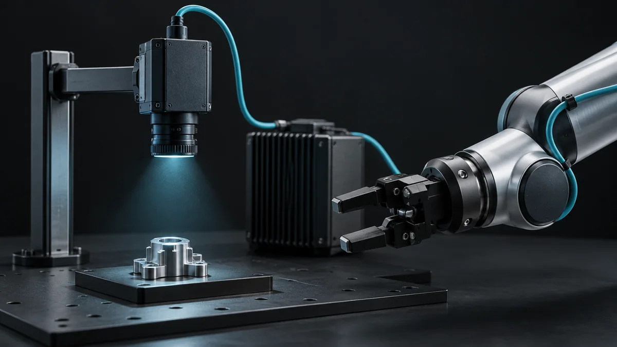
Use timestamped logs from a replay pipeline or bench camera. Identify whether each timestamp marks exposure start, end or delivery.
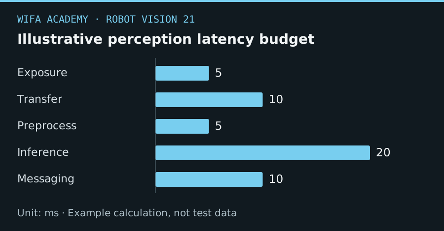
Read the diagram as a data table
| Condition or component | ms |
|---|---|
| Exposure | 5 |
| Transfer | 10 |
| Preprocess | 5 |
| Inference | 20 |
| Messaging | 10 |
The calculation
t_total = Σt_stage
e_motion = v_object × t_total
Times are seconds and object speed is mm/s. The position-error estimate assumes constant object velocity and no prediction.
Worked example
An illustrative pipeline of 5 ms exposure, 10 ms transfer, 5 ms preprocessing, 20 ms inference and 10 ms messaging totals 50 ms. At 200 mm/s, a part travels 10 mm during that delay.
Try it step by step
- Instrument each stage with a suitable monotonic clock and identify any asynchronous buffering or queueing.
- Measure distributions over many frames, including slow cases and dropped frames, rather than reporting only a mean.
- Attach capture time to every target and reject stale results before they reach the motion planner.
- Compare image-time target position with expected intercept position and validate any prediction using recorded motion.
How to check the result
Report capture-to-decision age and its high-percentile values alongside model inference time. Confirm that the clocks share a valid time reference.
Common mistake to avoid
Adding average stage times can hide queue buildup. A high throughput pipeline can still deliver old images.
Reference reading
Primary references for the underlying models, APIs or application context. The worked numbers and plots above are educational calculations, not results reported by these sources.