What you need
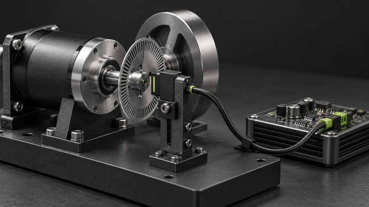
Use recorded encoder counts with monotonic timestamps and a known decoded count-per-revolution value.
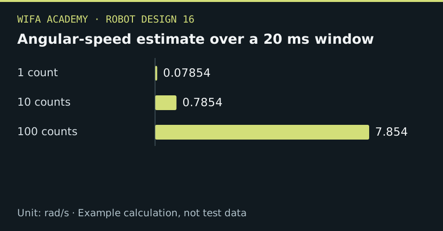
Read the diagram as a data table
| Condition or component | rad/s |
|---|---|
| 1 count | 0.07854 |
| 10 counts | 0.7854 |
| 100 counts | 7.854 |
The calculation
ω = 2π × Δcounts / (N_counts × Δt)
ω is rad/s, N_counts is decoded counts/revolution and Δt is seconds. Apply gearing if the sensor is not on the output joint.
Worked example
A change of 100 counts over 0.02 s with 4,000 counts/revolution gives 7.854 rad/s, or 75 rpm. At the same window length, one count corresponds to 0.07854 rad/s, illustrating quantization at low speeds.
Try it step by step
- Verify count scale and direction with a known rotation, then define rollover-safe differences for the counter width.
- Use measured elapsed time rather than assuming every loop executes at the nominal period.
- Compare fixed-window count differences with period-based methods if very low speed matters.
- Test acceleration and reversal sequences offline before choosing filtering and control-loop integration.
How to check the result
The estimate should remain well-defined at zero speed and across rollover, with documented latency and low-speed resolution.
Common mistake to avoid
Differentiating noisy position directly can create large spikes. An apparently smooth estimate may hide substantial filter delay.
Reference reading
Primary references for the underlying models, APIs or application context. The worked numbers and plots above are educational calculations, not results reported by these sources.