What you need
Use a plant model or identified response and a timing trace of the planned controller. Perform stability analysis before hardware tuning.
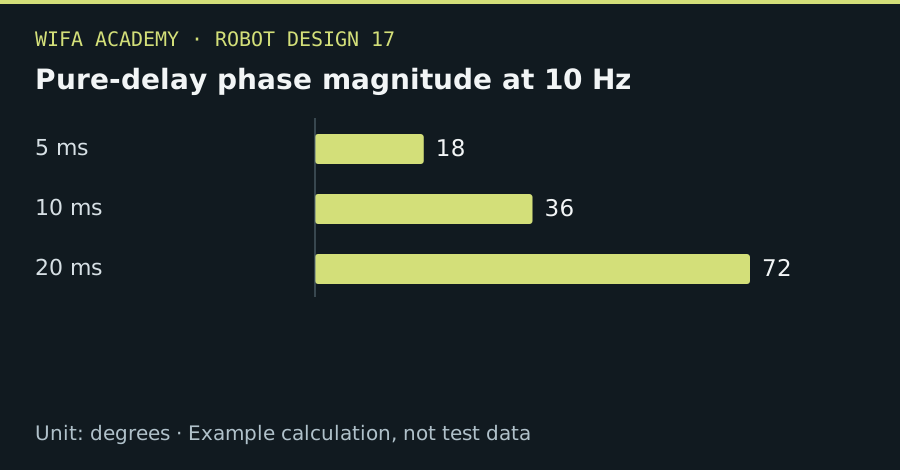
Read the diagram as a data table
| Condition or component | degrees |
|---|---|
| 5 ms | 18 |
| 10 ms | 36 |
| 20 ms | 72 |
The calculation
T_sample = 1 / f_sample
phase_delay = −ω × T_delay
The delay phase is radians at angular frequency ω in rad/s. It describes a pure delay and does not include the plant or controller phase.
Worked example
At a 10 Hz motion frequency, ω=62.83 rad/s. A 5 ms delay adds about -18° phase; 20 ms adds -72°. Two systems with the same nominal sample rate can behave differently if their total delays differ.
Try it step by step
- Identify the motion bandwidth you need and the plant dynamics that limit achievable control performance.
- Measure the complete sensor-to-actuator delay and jitter, including communication and filtering.
- Choose a sampling rate and controller using a proper discrete-time or delay-aware design, then simulate disturbances and saturation.
- Verify actual timing under worst computational load before a cautious supervised tuning procedure.
How to check the result
Report loop period, worst-case execution time, latency and jitter separately; a requested timer rate is not evidence of delivered timing.
Common mistake to avoid
Sampling just above twice a signal frequency is not a practical universal recipe for stable robot control.
Reference reading
Primary references for the underlying models, APIs or application context. The worked numbers and plots above are educational calculations, not results reported by these sources.